In this adventure we wish to explore lemniscates.
When the graph of a product forms two loops connected at a single point a
lemniscate is formed. Let us first look at an example of a lemniscate so we can
get an idea of the object that we are studying. Consider the equation whose
graph is shown below.
![]()
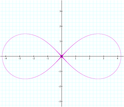
Many
students probably view form of the equation for this lemniscate as unappealing
and disgusting despite its obvious geometric appearance. We clearly see that this equation is
nothing more than the product of two circles, both with radius 3, with centers
(3,0) and (-3,0). Given the radius
and centers of these circles it is clear that the origin is the only point that
is on both circles and therefore it is no surprise that the origin is the point
of self-intersection of the graph.
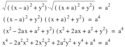
Is there a more concise or “pretty” form of this equation? Lets explore!
![]()
![]()
(x^2 - 6x +
9 + y^2)( x^2 + 6x + 9 + y^2) = 81
x^4 –
18 x^2 +2 x^2 y^2 +18 y^2 + y^4 + 81 = 81
![]()
![]()
![]()
This
form is much easier on the eyes, however, we can no longer see the connection
to circles. In the end we
sacrifice some intuition for visual appeal. Now we proceed explore the general case now that we have an
example to guide us.
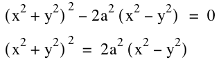
The
general case works exactly like the example did and so we have this nice
looking representation of the lemniscate with foci (a,0) and (-a,0). Lets plot the lemniscate for different
values of a. Notice that we only
need to try nonnegative values for a since our equation is symmetric in a and
–a. Let us plot for
a=2,1,1/2, and 0.
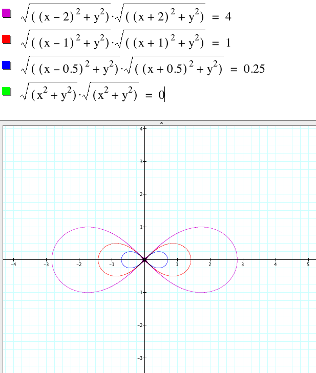
Notice
we have no green graph for the case where a=0. Acually when a=0 our graph is just one point, the
origin. Why is that? Well, from
above we have x^2 + y^2 =0 which means we must have x=y=0 since x^2 >= 0 and
y^2 >= 0 for all real values of x and y and x^2 = 0 = y^2 only when x = 0 =
y. We can deduce from above that
for all nonzero a the lemniscate with foci (a,0) and (-a,0) are “essentially”
the same with a=0 being a singularity case.
What
would happen if we were to vertically shift the left hand side of our “pretty”
equation? That is, what does the graph of
![]()
Look like for varying values of b? Let us graph this for b = 2 , 1 , 0 , -1 , and -2, for a=2,
just to get an idea.
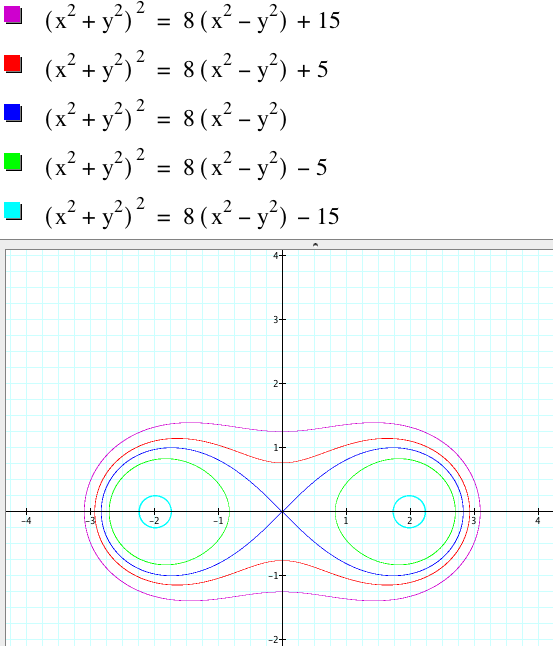
This
is interesting! As we shift
vertically up we move from two connected circles to a single figure which looks
as though could possibly approach a circle as b increases. As we shift vertically down we move
from two connected loops to two disconnected loops which appear to appear to be
converging to two points.
As
a last exploration, its is hard to ignore the clear relationships and
resemblences to circles so it is natural to think what this equation looks like
in polar coordinates. Recall: in
polar coordinates we have x = r*cos(q) and y =
r*sin(q). If r = 0 then this equation is trival, 0
= 0, so assume r is nonzero. Also
assume a is nonzero since that is the trival case where x = y = 0. Substituting
for x and y we have
![]()
((r*cos(q))^2 + (r*sin(q))^2)^2 =
2(a^2)((r*cos(q))^2 – (r*sin(q))^2)
((r^2)((cos(q))^2 + (sin(q))^2)^2 =
2(a^2)(r^2)((cos(q))^2 – (sin(q))^2)
((r^2)(1))^2
= 2(a^2)(r^2)cos(q/2)
r^4 =
2(a^2)(r^2)cos(q/2)
r^2 =
2(a^2)cos(q/2)
(r/a)^2 =
2cos(q/2).
This
is probably the most compact form for the lemniscate but this form also hides
the geometry of the lemniscate.
Certainly there is much more to explore with the lemniscate; more than
we can ever known. For example, we
could explore derivatives of the function with repect to x. What about computing the integral to
find area? What about other
transformations? Perhaps these
angles will be explored in the future.